合併重複行並對 Excel 中的值求和(簡單技巧)
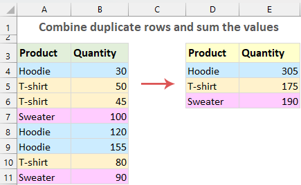
在 Excel 中,經常會遇到包含重複條目的資料集。 通常,您可能會發現自己擁有一系列數據,其中的關鍵挑戰是有效組合這些重複行,同時對相應列中的值進行求和,如下圖所示。 在此背景下,我們將深入研究幾種實用方法,這些方法可以幫助您合併重複資料並聚合其關聯值,從而增強 Excel 工作簿的清晰度和實用性。
合併重複的行並求和
合併重複行並使用 Consolidate 函數對值求和
合併是我們在 Excel 中合併多個工作表或行的有用工具,透過此功能,我們可以快速輕鬆地合併重複的行並彙總其相應的值。 請依照以下步驟進行:
第 1 步:選擇目標儲存格
選擇您希望合併資料出現的位置。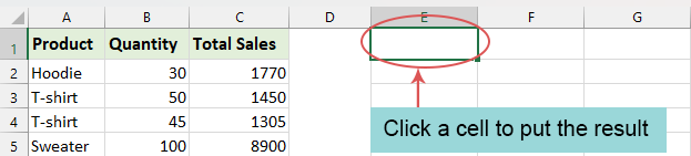
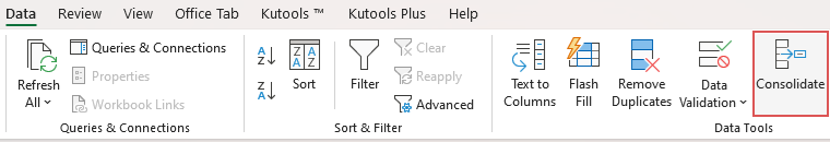
步驟 2:存取合併功能並設定合併
- 點擊 數據 > 整合,請參見屏幕截圖:
- 在 整合 對話框:
- (1.)選擇 總和 功能 下拉列表;
- (2.) 按一下以選擇要合併到的範圍 參數支持 框;
- (3.)檢查 第一排 和 左欄 在中使用標籤 選項;
- (4.) 最後,按一下 OK 按鈕。

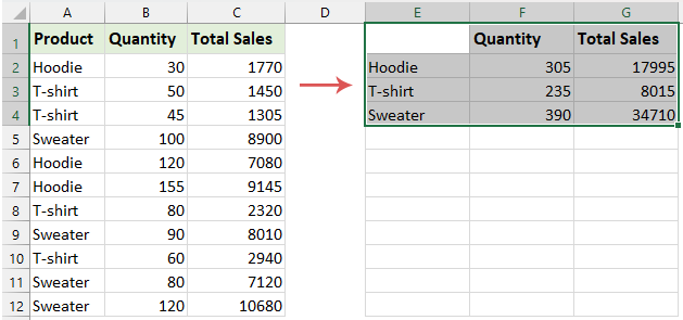
結果:
Excel 將合併第一列中找到的所有重複項,並將相鄰列中的對應值相加,如下圖所示:
- 如果範圍不包含標題行,請確保 取消選取頂行 來自 在中使用標籤 選項。
- 使用此功能,只能根據資料的第一列(最左邊)來合併計算。
合併重複的行並使用強大的功能對值求和 – Kutools
如果你已經安裝 Excel的Kutools,其 高級合併行 此功能可讓您輕鬆組合重複的行,提供資料求和、計數、平均或執行其他計算的選項。 此外,這項功能不僅限於一個鍵列,它還可以處理多個鍵列,使複雜的資料整合任務變得更加容易。
安裝後 Excel的Kutools,選擇資料範圍,然後按一下 庫工具 > 合併與拆分 > 高級合併行.
在 高級合併行 對話框中,請設置以下操作:
- 按一下您要根據其合併重複項的列名稱,在這裡,我將按一下“產品”,然後選擇 首要的關鍵 從下拉列表中 手術 柱;
- 然後,選擇要對值求和的列名稱,然後選擇 總和 從下拉列表中 手術 柱;
- 對於其他列,您可以選擇您需要的操作,例如將值與特定分隔符號組合或執行某種計算; (如果只有兩列,則可以忽略此步驟)
- 最後,您可以預覽合併結果,然後按一下 OK 按鈕。

結果:
現在,鍵列中的重複值被組合起來,其他對應的值被總結起來,如下圖所示:

- 透過這個有用的功能,您還可以根據重複的儲存格值合併行,如下所示:

- 此功能 支援撤銷,如果您想恢復原始數據,只需按 按Ctrl + Z.
- 要應用此功能,請 下載並安裝 Kutools for Excel 第一。
合併重複行並將數值與資料透視表相加
Excel 中的資料透視表提供了一種重新排列、分組和匯總資料的動態方式。 當您面對充滿重複條目的資料集並且需要對對應值求和時,此功能變得非常有用。
第 1 步:建立資料透視表
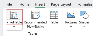
- 選擇數據範圍。 然後,轉到 插入 選項卡,然後單擊 數據透視表,請參見屏幕截圖:
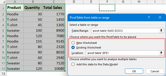
- 在彈出的對話方塊中,選擇資料透視表報表的放置位置,您可以根據需要將其放置到新工作表或現有工作表中。 然後,點擊 OK。 看截圖:
- 現在,資料透視表已插入到選取的目標儲存格中。 看截圖:

步驟 2:設定資料透視表:
- 在 數據透視表字段 窗格中,將包含重複項的欄位拖曳到 行 區域。 這將對您的重複項進行分組。
- 接下來,將包含要求和的值的欄位拖曳到 價值觀 區域。 預設情況下,Excel 會對值進行求和。 請參閱下面的演示:
結果:
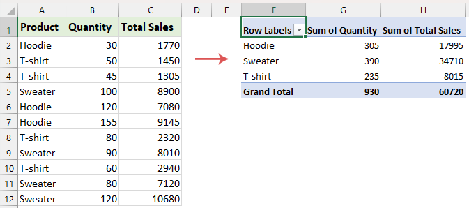
資料透視表現在顯示合併了重複項的資料及其總計值,為分析提供清晰簡潔的視圖。 看截圖:

合併重複的行並使用VBA代碼對值求和
如果您對 VBA 程式碼感興趣,在本節中,我們將提供一個 VBA 程式碼來合併重複行並對其他列中的對應值求和。 請依照以下步驟進行:
步驟1:開啟VBA工作表模組編輯器並複製程式碼
- 按住 ALT + F11 在Excel中打開鍵 Microsoft Visual Basic for Applications 窗口。
- 點擊 插入 > 模塊,然後將以下代碼粘貼到 模塊 窗口。
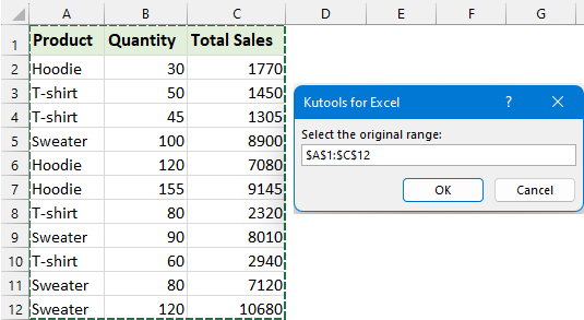
VBA代碼:合併重複的行並求和Sub CombineDuplicateRowsAndSumForMultipleColumns() 'Update by Extendoffice Dim SourceRange As Range, OutputRange As Range Dim Dict As Object Dim DataArray As Variant Dim i As Long, j As Long Dim Key As Variant Dim ColCount As Long Dim SumArray() As Variant Dim xArr As Variant Set SourceRange = Application.InputBox("Select the original range:", "Kutools for Excel", Type:=8) If SourceRange Is Nothing Then Exit Sub ColCount = SourceRange.Columns.Count Set OutputRange = Application.InputBox("Select a cell for output:", "Kutools for Excel", Type:=8) If OutputRange Is Nothing Then Exit Sub Set Dict = CreateObject("Scripting.Dictionary") DataArray = SourceRange.Value For i = 1 To UBound(DataArray, 1) Key = DataArray(i, 1) If Not Dict.Exists(Key) Then ReDim SumArray(1 To ColCount - 1) For j = 2 To ColCount SumArray(j - 1) = DataArray(i, j) Next j Dict.Add Key, SumArray Else xArr = Dict(Key) For j = 2 To ColCount xArr(j - 1) = xArr(j - 1) + DataArray(i, j) Next j Dict(Key) = xArr End If Next i OutputRange.Resize(Dict.Count, ColCount).ClearContents i = 1 For Each Key In Dict.Keys OutputRange.Cells(i, 1).Value = Key For j = 1 To ColCount - 1 OutputRange.Cells(i, j + 1).Value = Dict(Key)(j) Next j i = i + 1 Next Key Set Dict = Nothing Set SourceRange = Nothing Set OutputRange = Nothing End Sub
第2步:執行程式碼
- 粘貼此代碼後,請按 F5 鍵來運行此程式碼。 在提示方塊中選擇需要合併求和的資料範圍。 然後,點擊 OK.
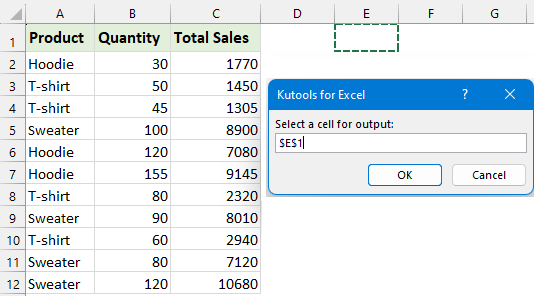
- 在接下來的提示方塊中,選擇要輸出結果的儲存格,然後按一下 OK.
結果:
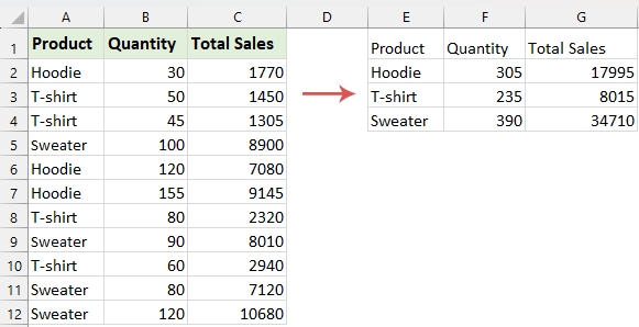
現在,重複的行被合併,並且它們對應的值已被求和。 看截圖:
在 Excel 中對重複行進行組合和求和既簡單又有效率。 從簡單的合併功能、進階的 Kutools、分析資料透視表或靈活的 VBA 編碼中進行選擇,以找到適合您的技能和需求的解決方案。 如果您有興趣探索更多 Excel 提示和技巧,我們的網站提供了數千個教程,請 點擊此處訪問它們。 感謝您的閱讀,我們期待在未來為您提供更多有用的信息!
相關文章:
- 根據重複項將多行合併為一行
- 也許,您有一系列數據,在產品名稱 A 列中,有一些重複的項目,現在您需要刪除 A 列中的重複條目,但合併 B 列中的相應值。如何在 Excel 中完成此任務?
- Vlookup並返回多個沒有重複的值
- 有時,您可能需要vlookup並將多個匹配的值一次返回到單個單元格中。 但是,如果在返回的單元格中填充了一些重複的值,那麼在返回所有匹配值時如何忽略重複項,而僅保留唯一值,如下面的Excel截圖所示?
- 合併具有相同 ID/名稱的行
- 例如,您有一個表格,如下圖所示,您需要將行與訂單ID合併,有什麼想法嗎? 在這裡,本文將為您介紹兩種解決方案。
最佳辦公生產力工具
| 🤖 | Kutools 人工智慧助手:基於以下內容徹底改變數據分析: 智慧執行 | 生成代碼 | 建立自訂公式 | 分析數據並產生圖表 | 呼叫 Kutools 函數... |
| 熱門特色: 尋找、突出顯示或識別重複項 | 刪除空白行 | 合併列或儲存格而不遺失數據 | 沒有公式的回合 ... | |
| 超級查詢: 多條件VLookup | 多值VLookup | 跨多個工作表的 VLookup | 模糊查詢 .... | |
| 高級下拉列表: 快速建立下拉列表 | 依賴下拉列表 | 多選下拉列表 .... | |
| 欄目經理: 新增特定數量的列 | 移動列 | 切換隱藏列的可見性狀態 | 比較範圍和列 ... | |
| 特色功能: 網格焦點 | 設計圖 | 大方程式酒吧 | 工作簿和工作表管理器 | 資源庫 (自動文字) | 日期選擇器 | 合併工作表 | 加密/解密單元格 | 按清單發送電子郵件 | 超級濾鏡 | 特殊過濾器 (過濾粗體/斜體/刪除線...)... | |
| 前 15 個工具集: 12 文本 工具 (添加文本, 刪除字符,...) | 50+ 圖表 類型 (甘特圖,...) | 40+ 實用 公式 (根據生日計算年齡,...) | 19 插入 工具 (插入二維碼, 從路徑插入圖片,...) | 12 轉化 工具 (數字到單詞, 貨幣兌換,...) | 7 合併與拆分 工具 (高級合併行, 分裂細胞,...) | ... 和更多 |
使用 Kutools for Excel 增強您的 Excel 技能,體驗前所未有的效率。 Kutools for Excel 提供了 300 多種進階功能來提高生產力並節省時間。 點擊此處獲取您最需要的功能...
")
Office選項卡為Office帶來了選項卡式界面,使您的工作更加輕鬆
- 在Word,Excel,PowerPoint中啟用選項卡式編輯和閱讀,發布者,Access,Visio和Project。
- 在同一窗口的新選項卡中而不是在新窗口中打開並創建多個文檔。
- 將您的工作效率提高 50%,每天為您減少數百次鼠標點擊!
")