如何在Excel中使用複選框突出顯示單元格或行?
如下圖所示,您需要選中復選框來突出顯示行或單元格。 選中復選框後,指定的行或單元格將自動突出顯示。 但是如何在Excel中實現呢? 本文將向您展示兩種實現方法。

使用條件格式複選框突出顯示單元格或行
用帶有VBA代碼的複選框突出顯示單元格或行
使用條件格式複選框突出顯示單元格或行
您可以創建條件格式規則,以在Excel中使用複選框突出顯示單元格或行。 請執行以下操作。
將所有復選框鏈接到指定的單元格
1.您需要通過單擊將復選框手動逐一插入到單元格中 開發者 > 插入 > 複選框 (表單控制).
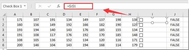
2.現在,複選框已插入到I列中的單元格。請選中I1中的第一個複選框,輸入公式 = $ J1 進入編輯欄,然後按 Enter 鍵。
尖端:如果您不想讓相鄰單元格中的值與復選框相關聯,則可以將復選框鏈接到另一個工作表的單元格,例如 = Sheet3!$ E1.
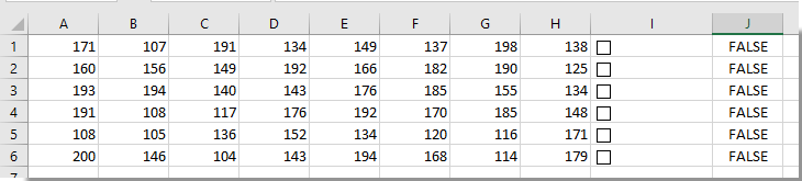
2.重複步驟1,直到所有復選框都鏈接到相鄰的單元格或另一個工作表中的單元格。
備註:所有鏈接的單元格應該是連續的,並且位於同一列中。
創建條件格式設置規則
現在,您需要按以下步驟創建條件格式設置規則。
1.選中需要用複選框突出顯示的行,然後單擊 條件格式 > 新規則 在 首頁 標籤。 看截圖:

2。 在裡面 新格式規則 對話框,您需要:
2.1選擇 使用公式來確定要格式化的單元格 在選項 選擇規則類型 框;
2.2輸入公式 = IF($ J1 = TRUE,TRUE,FALSE) 到 格式化此公式為真的值 框;
Or = IF(Sheet3!$ E1 = TRUE,TRUE,FALSE) 如果復選框鏈接到另一個工作表。
2.3點擊 格式 按鈕為行指定突出顯示的顏色;
2.4點擊 OK 按鈕。 看截圖:

備註: 在公式, $ J1 or $ E1 是複選框的第一個鏈接單元格,並確保單元格引用已更改為絕對列(J1> $ J1 or E1> $ E1).
現在,將創建條件格式設置規則。 選中復選框時,相應的行將自動突出顯示,如下圖所示。

用帶有VBA代碼的複選框突出顯示單元格或行
以下VBA代碼還可以幫助您在Excel中使用複選框突出顯示單元格或行。 請執行以下操作。
1.在工作表中,您需要突出顯示帶有復選框的單元格或行。 右鍵點擊 工作表標籤 並選擇 查看代碼 從右鍵菜單中打開 Microsoft Visual Basic for Applications 窗口。
2.然後將下面的VBA代碼複製並粘貼到“代碼”窗口中。
VBA代碼:在Excel中用複選框突出顯示行
Sub AddCheckBox()
Dim xCell As Range
Dim xRng As Range
Dim I As Integer
Dim xChk As CheckBox
On Error Resume Next
InputC:
    Set xRng = Application.InputBox("Please select the column range to insert checkboxes:", "Kutools for Excel", Selection.Address, , , , , 8)
If xRng Is Nothing Then Exit Sub
If xRng.Columns.Count > 1 Then
    MsgBox "The selected range should be a single column", vbInformation, "Kutools fro Excel"
    GoTo InputC
Else
    If xRng.Columns.Count = 1 Then
        For Each xCell In xRng
            With ActiveSheet.CheckBoxes.Add(xCell.Left, _
               xCell.Top, xCell.Width = 15, xCell.Height = 12)
               .LinkedCell = xCell.Offset(, 1).Address(External:=False)
               .Interior.ColorIndex = xlNone
               .Caption = ""
               .Name = "Check Box " & xCell.Row
            End With
            xRng.Rows(xCell.Row).Interior.ColorIndex = xlNone
        Next
    End If
    With xRng
     .Rows.RowHeight = 16
    End With
    xRng.ColumnWidth = 5#
    xRng.Cells(1, 1).Offset(0, 1).Select
    For Each xChk In ActiveSheet.CheckBoxes
      xChk.OnAction = ActiveSheet.Name + ".InsertBgColor"
    Next
End If
End Sub

Sub InsertBgColor()
Dim xName As Integer
Dim xChk As CheckBox
For Each xChk In ActiveSheet.CheckBoxes
  xName = Right(xChk.Name, Len(xChk.Name) - 10)
  If (xName = Range(xChk.LinkedCell).Row) Then
   If (Range(xChk.LinkedCell) = "True") Then
    Range("A" & xName, Range(xChk.LinkedCell).Offset(0, -2)).Interior.ColorIndex = 6
   Else
    Range("A" & xName, Range(xChk.LinkedCell).Offset(0, -2)).Interior.ColorIndex = xlNone
   End If
  End If
Next
End Sub
3。 按 F5 鍵來運行代碼。 (備註:您應將光標置於代碼的第一部分以應用F5鍵)在彈出窗口中 Excel的Kutools 對話框,請選擇要插入的範圍複選框,然後單擊 OK 按鈕。 在這裡,我選擇範圍I1:I6。 看截圖:

4.然後將復選框插入到選定的單元格中。 選中任何一個複選框,對應的行將自動突出顯示,如下圖所示。

相關文章:
- 在Excel中選中復選框時,如何更改指定的單元格值或顏色?
- 如果在Excel中選中復選框,如何在單元格中插入日期戳?
- 如何根據Excel中的單元格值選中復選框?
- 如何基於Excel中的複選框過濾數據?
- 在Excel中隱藏行時如何隱藏複選框?
- 如何在Excel中創建帶有多個複選框的下拉列表?
最佳辦公生產力工具
| 🤖 | Kutools 人工智慧助手:基於以下內容徹底改變數據分析: 智慧執行 | 生成代碼 | 建立自訂公式 | 分析數據並產生圖表 | 呼叫 Kutools 函數... |
| 熱門特色: 尋找、突出顯示或識別重複項 | 刪除空白行 | 合併列或儲存格而不遺失數據 | 沒有公式的回合 ... | |
| 超級查詢: 多條件VLookup | 多值VLookup | 跨多個工作表的 VLookup | 模糊查詢 .... | |
| 高級下拉列表: 快速建立下拉列表 | 依賴下拉列表 | 多選下拉列表 .... | |
| 欄目經理: 新增特定數量的列 | 移動列 | 切換隱藏列的可見性狀態 | 比較範圍和列 ... | |
| 特色功能: 網格焦點 | 設計圖 | 大方程式酒吧 | 工作簿和工作表管理器 | 資源庫 (自動文字) | 日期選擇器 | 合併工作表 | 加密/解密單元格 | 按清單發送電子郵件 | 超級濾鏡 | 特殊過濾器 (過濾粗體/斜體/刪除線...)... | |
| 前 15 個工具集: 12 文本 工具 (添加文本, 刪除字符,...) | 50+ 圖表 類型 (甘特圖,...) | 40+ 實用 公式 (根據生日計算年齡,...) | 19 插入 工具 (插入二維碼, 從路徑插入圖片,...) | 12 轉化 工具 (數字到單詞, 貨幣兌換,...) | 7 合併與拆分 工具 (高級合併行, 分裂細胞,...) | ... 和更多 |
使用 Kutools for Excel 增強您的 Excel 技能,體驗前所未有的效率。 Kutools for Excel 提供了 300 多種進階功能來提高生產力並節省時間。 點擊此處獲取您最需要的功能...
")
Office選項卡為Office帶來了選項卡式界面,使您的工作更加輕鬆
- 在Word,Excel,PowerPoint中啟用選項卡式編輯和閱讀,發布者,Access,Visio和Project。
- 在同一窗口的新選項卡中而不是在新窗口中打開並創建多個文檔。
- 將您的工作效率提高 50%,每天為您減少數百次鼠標點擊!
")