在 Excel 中建立搜尋框 – 逐步指南
在 Excel 中建立搜尋框可以更輕鬆地快速篩選和存取特定數據,從而增強電子表格的功能。本指南涵蓋了實作搜尋框的幾種方法,以適應不同版本的 Excel。無論您是初學者還是高級用戶,這些步驟都將幫助您使用 FILTER 函數、條件格式和各種公式等功能設定動態搜尋框。
- 輕鬆建立搜尋框 過濾器功能
(適用於 Excel 2019 及更高版本、Excel for Microsoft 365)
- 使用建立搜尋框 條件格式
(適用於所有 Excel 版本)
- 建立一個搜尋框 配方組合
(適用於所有 Excel 版本)
使用FILTER功能輕鬆建立搜尋框
- 當資料發生變化時,此函數會自動更新輸出。
- FILTER 函數可以傳回任意數量的結果,從單行到數千行,這取決於資料集中有多少條目符合您設定的條件。
下面我將向您展示如何使用FILTER函數在Excel中建立搜尋框。
步驟1:插入文字方塊並配置屬性
- 轉到 開發者
標籤,點擊 插入 > T外部框(ActiveX 控制項).
尖端:如果 開發者 選項卡未顯示在功能區上,您可以按照本教學中的說明啟用它: 如何在Excel功能區中顯示/顯示開發人員選項卡?

- 遊標將變成十字形,然後您需要拖曳遊標將文字方塊繪製在工作表中要放置文字方塊的位置。繪製文字方塊後,釋放滑鼠。

- 右鍵單擊文字方塊並選擇 氟化鈉性能 從上下文菜單。

- 在 氟化鈉性能 窗格中,透過在文字方塊中輸入儲存格參考將文字方塊連結到儲存格 鏈接單元 場地。例如,輸入“J2" 確保在文字方塊中輸入的任何資料都會在儲存格 J2 中自動更新,反之亦然。

- 點擊 設計模式 在 開發者
選項卡退出設計模式。

文字方塊現在允許您輸入文字。
步驟 2:應用 FILTER 功能
- 在使用FILTER功能之前,請將原始標題行複製到新區域。在這裡,我將標題行放置在搜尋框下方。
尖端:這種方法允許使用者在與原始資料相同的列標題下清楚地看到結果。

- 選擇第一個標題下的儲存格(例如 I5 在此範例中),輸入以下公式並按 Enter 獲得結果的關鍵。
=FILTER(Sheet2!$A$5:$G$281,Sheet2!$B$5:$B$281=J2,"No data found") 如上面的截圖所示,由於文字方塊現在沒有輸入,所以公式顯示結果“沒有找到數據“中 I5.
- 在這個公式中:
- 表 2!:$A$5:$G$281是Sheet2上要過濾的資料範圍。
- Sheet2!$B$5:$B$281=J2:這部分定義用於過濾範圍的標準。它檢查 Sheet5 上第 281 行到第 2 行 B 列中的每個儲存格,看看它是否等於儲存格 J2 中的值。 J2 是連結到搜尋框的儲存格。
- 沒有找到數據:如果FILTER函數沒有找到任何B列中的值等於單元格J2中的值的行,它將傳回「找不到資料」。
- 這個方法是 不區分大小寫,這意味著無論您輸入大寫字母還是小寫字母,它都會匹配文字。
結果:測試搜尋框
現在讓我們測試一下搜尋框。在這個例子中,當我在搜尋框中輸入客戶姓名時,相應的結果將立即被過濾並顯示。

使用條件格式建立搜尋框
條件格式可用於突出顯示與搜尋詞相符的數據,從而間接建立搜尋框效果。此方法不會過濾掉數據,而是直觀地引導您找到相關單元格。本節將向您展示如何使用 Excel 中的條件格式建立搜尋框。
步驟1:插入文字方塊並配置屬性
- 轉到 開發者
標籤,點擊 插入 > T外部框(ActiveX 控制項).
尖端:如果 開發者 選項卡未顯示在功能區上,您可以按照本教學中的說明啟用它: 如何在Excel功能區中顯示/顯示開發人員選項卡?
- 遊標將變成十字形,然後您需要拖曳遊標將文字方塊繪製在工作表中要放置文字方塊的位置。繪製文字方塊後,釋放滑鼠。
- 右鍵單擊文字方塊並選擇 氟化鈉性能 從上下文菜單。
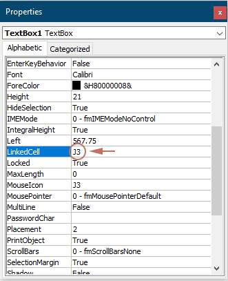
- 在 氟化鈉性能 窗格中,透過在文字方塊中輸入儲存格參考將文字方塊連結到儲存格 鏈接單元 場地。例如,輸入“J3" 確保在文字方塊中輸入的任何資料都會在儲存格 J3 中自動更新,反之亦然。
- 點擊 設計模式 在 開發者
選項卡退出設計模式。
文字方塊現在允許您輸入文字。
步驟 2:應用條件格式來搜尋數據
- 選擇要搜尋的整個資料範圍。這裡我選擇範圍A3:G279。
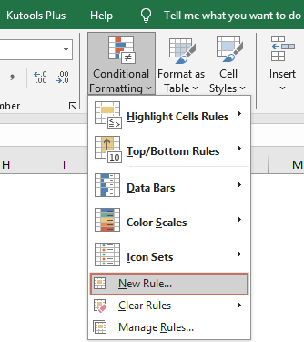
- 下 首頁
標籤,點擊 條件格式 > 新規則.
- 在 新格式規則 對話框:
- 選擇 使用公式來確定要格式化的單元格 ,在 選擇規則類型 選項。
- 將以下公式輸入到 格式化此公式為真的值 框。
=$B3=$J$3在這裡, $ B3 表示要與選取範圍內的搜尋條件相符的資料列中的第一個儲存格,以及 $J$3 是連結到搜尋框的儲存格。 - 點擊 格式 按鈕指定搜尋結果的填滿顏色。
- 點擊 OK 按鈕。 看截圖:

結果
現在讓我們測試一下搜尋框。在此範例中,當我在搜尋框中輸入客戶姓名時,B 列中包含該客戶的相應行將立即使用指定的填滿色彩突出顯示。
建立包含公式組合的搜尋框
如果您沒有使用最新版本的 Excel 並且不希望僅突出顯示行,本節中描述的方法可能會有所幫助。您可以使用 Excel 公式的組合在任何版本的 Excel 中建立功能搜尋框。請依照以下步驟操作。
步驟 1:從搜尋列建立唯一值列表
- 在本例中,我選擇並複製範圍 B4:B281 到一個新的工作表。
- 將範圍貼到新工作表中後,保持所選貼上的數據,轉到 數據 選項卡並選擇 刪除重複項.

- 在開 刪除重複項 對話框中,單擊 OK 按鈕。
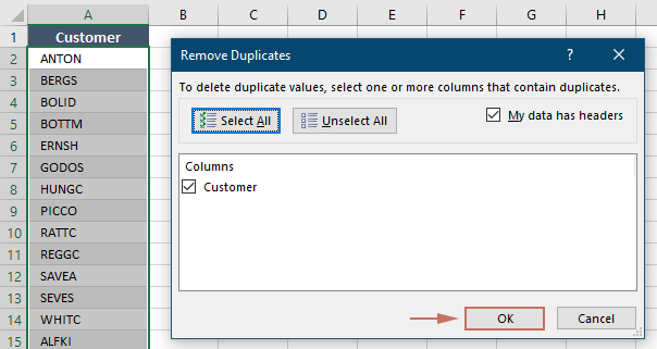
- A Microsoft Excel中 然後彈出提示框,顯示刪除了多少重複。點選 OK.

- 刪除重複項後,選擇清單中的所有唯一值(不包括標題),並透過在 姓名 盒子。這裡我將範圍命名為 客戶.

步驟 2:插入組合方塊並配置屬性
- 返回包含要搜尋的資料集的工作表。前往 開發者
標籤,點擊 插入 > 組合框(ActiveX控件).
尖端:如果 開發者 選項卡未顯示在功能區上,您可以按照本教學中的說明啟用它: 如何在Excel功能區中顯示/顯示開發人員選項卡?

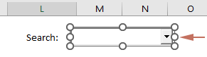
- 遊標將變成十字形,然後您需要拖曳遊標在工作表中要放置搜尋框的位置繪製組合框。繪製組合框後,放開滑鼠。
- 右鍵單擊組合框並選擇 氟化鈉性能 從上下文菜單。

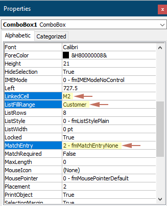
- 在 氟化鈉性能 窗格:
- 透過在儲存格引用中輸入儲存格引用,將組合方塊連結到儲存格 鏈接單元 場地。她我輸入“M2".
提示:指定此欄位可確保在組合方塊中輸入的任何資料都會在儲存格 M2 中自動更新,反之亦然。
- 在 列表填充範圍 字段,輸入 範圍名稱 您在步驟 1 中指定了唯一清單。
- 更改 匹配項 字段 2 – fmMatchEntryNone.
- 關上 氟化鈉性能 窗格。
- 透過在儲存格引用中輸入儲存格引用,將組合方塊連結到儲存格 鏈接單元 場地。她我輸入“M2".
- 點擊 設計模式 在 開發者
選項卡退出設計模式。
現在您可以從組合方塊中選擇任何項目或輸入要搜尋的文字。
第 3 步:應用公式
- 建立與原始資料範圍相鄰的三個輔助列。看截圖:

- 在單元格中(H5)在第一個輔助列的標題下,輸入以下公式並按 Enter.
=ROWS($B$5:B5)這裡 B5 是包含要搜尋的欄位的第一個客戶名稱的儲存格。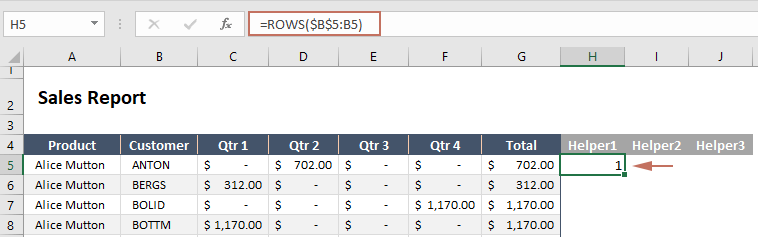
- 雙擊右下角的公式單元格,後面的儲存格會自動填入相同的公式。
- 在單元格中(I5)在第二個輔助列標題下,輸入以下公式並按 Enter。然後雙擊公式單元格的右下角,自動用相同的公式填充下面的單元格。
=IF(ISNUMBER(SEARCH($M$2,B5)),H5,"")這裡 M2 是鏈接到組合框的單元格。
- 在單元格中(J5)在第三個輔助列標題下,輸入以下公式並按 Enter。然後雙擊公式單元格的右下角,自動用相同的公式填充下面的單元格。
=IFERROR(SMALL($I$5:$I$281,H5),"")
- 將原始標題行複製到新區域。在這裡,我將標題行放置在搜尋框下方。
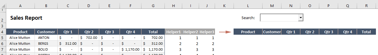
- 選擇第一個標題下的儲存格(例如 L5 在本例中),輸入下列公式並按 Enter 鍵。
=IFERROR(INDEX($A$5:$G$281,$J5,COLUMNS($L$4:L4)),"")這裡 A5:G281 是您想要在結果儲存格中顯示的整個資料範圍。
- 選擇該公式單元格,拖曳 填充手柄 向右然後向下將公式套用到對應的列和行。
 筆記:
筆記:- 由於搜尋框中沒有輸入,公式的結果將顯示原始資料。
- 此方法不區分大小寫,這意味著無論您輸入大寫字母還是小寫字母,它都會匹配文字。
結果
現在讓我們測試一下搜尋框。在此範例中,當我從組合方塊中輸入或選擇客戶名稱時,B 列中包含該客戶名稱的相應行將被過濾並立即顯示在結果範圍中。

在 Excel 中建立搜尋框可以顯著改善您與資料的互動方式,讓您的電子表格更加動態且使用者友好。無論您選擇簡單的 FILTER 函數、條件格式的視覺輔助,還是選擇多功能的公式組合,每種方法都提供了寶貴的工具來增強您的資料操作能力。嘗試這些技術,找出最適合您的特定需求和資料場景的技術。對於那些渴望深入研究 Excel 功能的人,我們的網站擁有豐富的教學。 在這裡了解更多 Excel 提示和技巧.
最佳辦公生產力工具
| 🤖 | Kutools 人工智慧助手:基於以下內容徹底改變數據分析: 智慧執行 | 生成代碼 | 建立自訂公式 | 分析數據並產生圖表 | 呼叫 Kutools 函數... |
| 熱門特色: 尋找、突出顯示或識別重複項 | 刪除空白行 | 合併列或儲存格而不遺失數據 | 沒有公式的回合 ... | |
| 超級查詢: 多條件VLookup | 多值VLookup | 跨多個工作表的 VLookup | 模糊查詢 .... | |
| 高級下拉列表: 快速建立下拉列表 | 依賴下拉列表 | 多選下拉列表 .... | |
| 欄目經理: 新增特定數量的列 | 移動列 | 切換隱藏列的可見性狀態 | 比較範圍和列 ... | |
| 特色功能: 網格焦點 | 設計圖 | 大方程式酒吧 | 工作簿和工作表管理器 | 資源庫 (自動文字) | 日期選擇器 | 合併工作表 | 加密/解密單元格 | 按清單發送電子郵件 | 超級濾鏡 | 特殊過濾器 (過濾粗體/斜體/刪除線...)... | |
| 前 15 個工具集: 12 文本 工具 (添加文本, 刪除字符,...) | 50+ 圖表 類型 (甘特圖,...) | 40+ 實用 公式 (根據生日計算年齡,...) | 19 插入 工具 (插入二維碼, 從路徑插入圖片,...) | 12 轉化 工具 (數字到單詞, 貨幣兌換,...) | 7 合併與拆分 工具 (高級合併行, 分裂細胞,...) | ... 和更多 |
使用 Kutools for Excel 增強您的 Excel 技能,體驗前所未有的效率。 Kutools for Excel 提供了 300 多種進階功能來提高生產力並節省時間。 點擊此處獲取您最需要的功能...
")
Office選項卡為Office帶來了選項卡式界面,使您的工作更加輕鬆
- 在Word,Excel,PowerPoint中啟用選項卡式編輯和閱讀,發布者,Access,Visio和Project。
- 在同一窗口的新選項卡中而不是在新窗口中打開並創建多個文檔。
- 將您的工作效率提高 50%,每天為您減少數百次鼠標點擊!
")