跳到主要內容

如何在Excel中基於一個或多個條件返回多個匹配值?

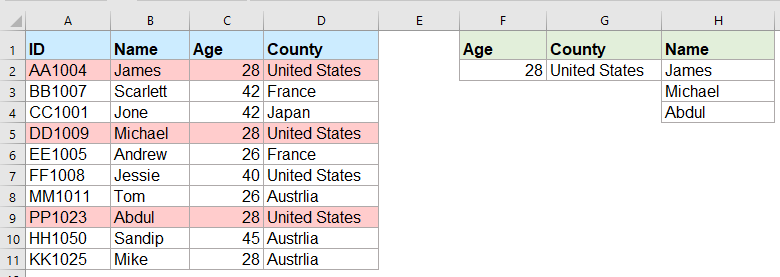
通常,對於大多數人來說,使用VLOOKUP函數查找特定值並返回匹配項很容易。 但是,您是否曾經嘗試過根據一個或多個條件返回多個匹配值,如下面的屏幕截圖所示? 在本文中,我將介紹一些解決Excel中復雜任務的公式。

根據一個或多個條件使用數組公式返回多個匹配值


根據一個或多個條件使用數組公式返回多個匹配值

例如,我要提取年齡為28歲且來自美國的所有姓名,請使用以下公式:

1。 將以下公式複製或輸入到要查找結果的空白單元格中:

=INDEX($B$2:$B$11, SMALL(IF(COUNTIF($F$2, $C$2:$C$11)*COUNTIF($G$2, $D$2:$D$11), ROW($A$2:$D$11)-MIN(ROW($A$2:$D$11))+1), ROW(A1)), COLUMN(A1))

備註:在以上公式中, B2:B11 是從中返回匹配值的列; F2, C2:C11 是第一個條件和包含第一個條件的列數據; G2, D2:D11 是第二個條件,包含此條件的列數據,請根據需要進行更改。

2。 然後按 Ctrl + Shift + Enter 鍵以獲取第一個匹配結果,然後選擇第一個公式單元格並將填充手柄向下拖動到這些單元格,直到顯示錯誤值,現在,所有匹配值都將返回,如下圖所示:

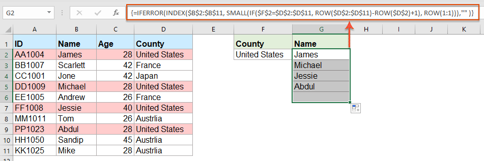
保養竅門:如果只需要根據一種條件返回所有匹配值,請應用以下數組公式:

=IFERROR(INDEX($B$2:$B$11, SMALL(IF($F$2=$D$2:$D$11, ROW($D$2:$D$11)-ROW($D$2)+1), ROW(1:1))),"" )


更多相關文章:

  • 在一個逗號分隔的單元格中返回多個查找值
  • 在Excel中,我們可以應用VLOOKUP函數從表單元格返回第一個匹配的值,但是有時,我們需要提取所有匹配的值,然後用特定的定界符(例如逗號,破折號等)分隔為單個單元格如下圖所示。 我們如何在Excel中的一個逗號分隔的單元格中獲取並返回多個查找值?
  • Vlookup並在Google表格中一次返回多個匹配值
  • Google表格中的常規Vlookup函數可以幫助您根據給定的數據查找並返回第一個匹配值。 但是,有時,您可能需要vlookup並返回所有匹配的值,如下圖所示。 您是否有任何簡便的方法可以解決Google表格中的此任務?
  • Vlookup並從下拉列表中返回多個值
  • 在Excel中,如何從下拉列表中進行vlookup並返回多個相應的值,這意味著當您從下拉列表中選擇一項時,其所有相對值會立即顯示,如以下屏幕截圖所示。 本文,我將逐步介紹解決方案。
  • Vlookup並在Excel中垂直返回多個值
  • 通常,您可以使用Vlookup函數來獲取第一個對應的值,但是有時,您希望基於特定條件返回所有匹配的記錄。 在本文中,我將討論如何進行vlookup並將所有匹配值垂直,水平或返回到單個單元格中。
  • Vlookup並在Excel中返回兩個值之間的匹配數據
  • 在Excel中,我們可以應用常規的Vlookup函數根據給定的數據獲取相應的值。 但是,有時,我們想要vlookup並返回兩個值之間的匹配值,如下面的屏幕截圖所示,您如何在Excel中處理此任務?


  • 超級公式欄 (輕鬆編輯多行文本和公式); 閱讀版式 (輕鬆讀取和編輯大量單元格); 粘貼到過濾範圍...
  • 合併單元格/行/列 和保存數據; 拆分單元格內容; 合併重複的行和總和/平均值...防止細胞重複; 比較範圍...
  • 選擇重複或唯一 行; 選擇空白行 (所有單元格都是空的); 超級查找和模糊查找 在許多工作簿中; 隨機選擇...
  • 確切的副本 多個單元格,無需更改公式參考; 自動創建參考 到多張紙; 插入項目符號,複選框等...
  • 收藏并快速插入公式,範圍,圖表和圖片; 加密單元 帶密碼 創建郵件列表 並發送電子郵件...
  • 提取文字,添加文本,按位置刪除, 刪除空間; 創建和打印分頁小計; 在單元格內容和註釋之間轉換...
  • 超級濾鏡 (將過濾方案保存並應用於其他工作表); 高級排序 按月/週/日,頻率及更多; 特殊過濾器 用粗體,斜體...
  • 結合工作簿和工作表; 根據關鍵列合併表; 將數據分割成多個工作表; 批量轉換xls,xlsx和PDF...
  • 數據透視表分組依據 週號,週幾等 顯示未鎖定的單元格 用不同的顏色 突出顯示具有公式/名稱的單元格...
kte選項卡201905
  • 在Word,Excel,PowerPoint中啟用選項卡式編輯和閱讀,發布者,Access,Visio和Project。
  • 在同一窗口的新選項卡中而不是在新窗口中打開並創建多個文檔。
  • 將您的工作效率提高 50%,每天為您減少數百次鼠標點擊!
officetab底部


Comments (25)
No ratings yet. Be the first to rate!
This comment was minimized by the moderator on the site
Hi, if there are duplicate values (e.g. two adams), how do i make sure that it only returns 1 adam and not 2?
This comment was minimized by the moderator on the site
Hello, Bobby,
To extract only unique matching values, you should apply the below formula:
After pasting the formula, please press Ctrl + Shift + Enter keys together to get the correct result.
=IFERROR(INDEX($B$2:$B$5, MATCH(0, COUNTIF(H1:$H$1, $B$2:$B$5)+IF($D$2:$D$5<>$G$2, 1, 0)+IF($C$2:$C$5<>$F$2, 1, 0), 0)), "")

Please have a try, hope it can help you!
This comment was minimized by the moderator on the site
Hi,

Thanks for posting these examples.
I'm trying to implement this in my own sheet, but don't get it to work (maybe because I'm using an europe version of excel)?

I want to get the dates of the days that I had my shifts or that I have worked 'some' (>0) hours for a client.

So in I3 is the name and in J3 the month. K3 and L3 are the shifts (1 is worked) and hours (don't know how to set this, should be more than zero)

My expected results are in:
Shifts: I7 and I8
hours: J7

So I worked more than 0 hours for 'person 2' in oktober on 3-10-2022
had shifts for person 2 on '10-10-2022' and 28-10-2022

When I add '=INDEX($B$2:$B$11, SMALL(IF(COUNTIF($F$2, $C$2:$C$11)*COUNTIF($G$2, $D$2:$D$11), ROW($A$2:$D$11)-MIN(ROW($A$2:$D$11))+1), ROW(A1)), COLUMN(A1))' in my excel sheet, it doesn't allow the comma between the different parts of the formula.
So I need to change them to ';'.
But when I try it it always says: '#NAME?'

So can someone help me with this?

Kind regards,

Bas
[img]https://drive.google.com/file/d/1iIPQKuj_PNhqWyWlwJ4IQTqGNEd6B9Hw/view?usp=share_link[/img]
This comment was minimized by the moderator on the site
Hi,

First, thank you for sharing!

Can you please provide a solution to the case below:

I have 3 columns (A: Containing reference information, B: Containing information to be searched, C: Search result)

Image url is provided below

https://ibb.co/VHCd09K

Column A-------------------------Column B------------Column C
File Name-------------------------Name----------------File Name, Document Name, Element Name, Name
Changed Element-----------------Element--------------Changed Element, Element Name, Element ID
Column Location
Document Name
Element Name
Name
Category
Warranty
Slope
Element ID

What I need is to search in column A for any partial match with cell B2 (Name) or B3 (Element) and get the result in one cell,

Thank you, Behzad
This comment was minimized by the moderator on the site
Hello, Behzad
Maybe the below User Defined Function can help you.
Public Function ConcatPartLookUp(rngInput As Range, rngSource As Range, Optional strDelimiter As String, Optional blCaseSensitive)
Dim rng As Range
If strDelimiter = "" Then strDelimiter = ","
If IsMissing(blCaseSensitive) Then
    blCaseSensitive = False
Else
    blCaseSensitive = True
End If
For Each rng In rngSource
    If blCaseSensitive Then
        If InStr(1, rng.Value, rngInput.Value, vbBinaryCompare) > 0 Then ConcatPartLookUp = ConcatPartLookUp & strDelimiter & rng.Value
    Else
        If InStr(1, rng.Value, rngInput.Value, vbTextCompare) > 0 Then ConcatPartLookUp = ConcatPartLookUp & strDelimiter & rng.Value
    End If
Next
If Len(ConcatPartLookUp) > 0 Then ConcatPartLookUp = Mid(ConcatPartLookUp, 2, Len(ConcatPartLookUp))
End Function


After copying and pasting this code, and then use this formula:=ConcatPartLookUp(B2,$A$2:$A$8) to get the result you need.
Please have a try, hope it can help you!
This comment was minimized by the moderator on the site
Heyi, thank you for the formula. It worked for "fixed" values / text as criterias. However, one of the criterias i'm trying to use is a condition (values <>0 ), but does not work the described formula. Do you guys know what should i change to adapt the formula so I can have a condition as one of the criterias, please?

Best,

João
This comment was minimized by the moderator on the site
Hello, Marcus
To solve your problem, please view this article:
https://www.extendoffice.com/documents/excel/6393-excel-vlookup-function.html#b3-2
There are some detailed explanations of this task. You just need to change the criteira to your own.
Thank you!
This comment was minimized by the moderator on the site
Hi,

if in cell H1 i write "Name" and wanted to link that with the formula, how would that work?
Then I could write "ID" in cell H1 and would automatically get as a result: AA1004; DD1009; PP1023 (for the first formula)

Thank you in advance!
This comment was minimized by the moderator on the site
Hello, Marie
Sorry, i can't get the point of your first problem, could you explain your problem more clearly and detailedly? Or you can insert a screenshot here to describe your problem.
As for the second question, you just need to change the cell reference as this:
=INDEX($A$2:$A$11, SMALL(IF(COUNTIF($F$2, $C$2:$C$11)*COUNTIF($G$2, $D$2:$D$11), ROW($A$2:$D$11)-MIN(ROW($A$2:$D$11))+1), ROW(A1)), COLUMN(A1))

Remeber to press Ctrl + Shift + Enter keys together.
Please try, hope it can help you!
This comment was minimized by the moderator on the site
Hello,
what would be needed to expand the first formula in the following case:
Some IDs are Blank (e.g. cell A5 is blank) and I would like an additional condition outputting lines only when the IDs are not blank. (So the output should then be James and Abdul.
Thanks!
This comment was minimized by the moderator on the site
Hello, Jo,
To solve your problem, please apply the below formula:
=INDEX($B$2:$B$11, SMALL(IF(COUNTIF($F$2, $C$2:$C$11)*COUNTIF($G$2, $D$2:$D$11)*($A$2:$A$11<>0), ROW($A$2:$D$11)-MIN(ROW($A$2:$D$11))+1), ROW(A1)), COLUMN(A1))

Please have a ry, hope it can help you!
This comment was minimized by the moderator on the site
hello,
ive tried using the formula and it either generates a value of 0 or the image attached
This comment was minimized by the moderator on the site
Hello, Milku
Your screenshot showed WPS software of MAC version, so I am not sure whether our formula is available.
I uploaded an Excel file to here, you can try to see if it can calculate correctly in you environment.
Thank you!
This comment was minimized by the moderator on the site
When I use the second formula and drag down, nothing appears. The formula result (fx) says it should be returning something but it is blank. How do I correct this?
This comment was minimized by the moderator on the site
Hello Alysia,

Glad to help. I tried the second formula in the article and drag the formula down, the rest of results were returned. I think there may be two reasons for your problem. First, maybe you forget to press Ctrl + Shift + Enter keys to enter the formula. Second, the matching result is only one, so no other results are not returned. Please have a check.

Sincerely,
Mandy
This comment was minimized by the moderator on the site
Hi,

I was wondering if it at all possible to enter a 2nd criteria but from the same range as the 1st criteria,

For example with the used example above i would like to search for the names of people from both America and France So cell F3 would have France, Scarlett & Andrew would also populate in the list in Column G

Thank you for assistance in advance.
This comment was minimized by the moderator on the site
Hello Nick,

Glad to help. If you want to get the names of people from both America and France, I advise you to use our formula twice to get the result. Please see the screenshot, In F2 and G2 are values "United States" and "France". Apply formula =IFERROR(INDEX($B$2:$B$11, SMALL(IF($F$2=$D$2:$D$11, ROW($D$2:$D$11)-ROW($D$2)+1), ROW(1:1))),"" ) to get the results for America. And apply formula =IFERROR(INDEX($B$2:$B$11, SMALL(IF($G$2=$D$2:$D$11, ROW($D$2:$D$11)-ROW($D$2)+1), ROW(1:1))),"" ) to get the results for France. It's simple. Please have a try.

Sincerely,
Mandy
This comment was minimized by the moderator on the site
In the first example, what change to the formula would be needed to return everyone who was less than 28 years old?
There are no comments posted here yet
Load More
Please leave your comments in English
Posting as Guest
×
Rate this post:
0   Characters
Suggested Locations