如何在 Excel 中顯示最高分對應的姓名？

作者Xiaoyang修改日期2025-10-10

當您在 Excel 中分析績效或成果時，經常需要從包含姓名與對應數值的資料集中找出誰獲得最高分。例如，您可能在一欄列出學生姓名，另一欄列出他們的測驗分數。此時不僅要找出最高分數，更要顯示取得該分數的所有人員姓名（若出現同分情況，則一併列出）。這種做法廣泛應用於追蹤頂尖銷售人員、學生成績、員工評估結果，或任何需要排名的情境。

以下提供幾種實用的解決方案，並附上清晰的逐步操作說明與實用提示，助您有效避開常見錯誤。請根據您的資料規模與報表需求，選擇最適合的方法。

使用公式顯示最高分對應的姓名

VBA 程式碼－自動找出並顯示最高分對應的姓名

資料透視表－使用資料透視表顯示最高分對應的姓名

使用公式顯示最高分對應的姓名

若要擷取最高分獲得者的姓名，下列公式可助您輕鬆達成。此方法特別適合中小型資料集，若您希望在不使用額外工具的情況下快速找出表現最佳者，效果尤佳。

若要找出最高分對應的姓名，請使用 INDEX 與 MATCH 函數組合，如下所示：

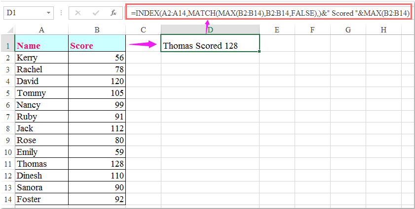
1. 在您要顯示姓名的空白儲存格中（例如 C2 儲存格），輸入下列公式：

=INDEX(A2:A14,MATCH(MAX(B2:B14),B2:B14,FALSE))&" Scored "&MAX(B2:B14)

輸入公式後，按下 Enter 確認。此公式會傳回所找到的第一個最高分對應的姓名。例如，若 John 與 Alice 同時取得 98 分，公式僅會傳回最先出現的名字。

輸入公式以顯示最高分對應的姓名

注意事項：

1. 在上述公式中，A2:A14 為您要擷取姓名的名稱清單，而 B2:B14 則為分數清單。請務必確認範圍與您的資料完全相符。
2. 此公式僅會傳回第一個符合條件的姓名。若有多人同為最高分，建議顯示所有相關姓名；詳見下方提供的實用解決方案。

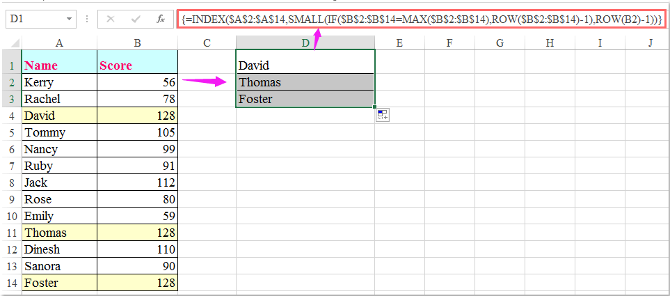
在任意儲存格中（例如 D2）輸入下列公式：

=INDEX($A$2:$A$14,SMALL(IF($B$2:$B$14=MAX($B$2:$B$14),ROW($B$2:$B$14)-1),ROW(B2)-1))

在輸入公式後，請同時按下 Ctrl + Shift + Enter（而非僅按 Enter），將其設為陣列公式，即可顯示最高分對應的姓名。接著選取該公式儲存格，向下拖曳填滿控點，持續拖曳直到出現錯誤值為止——每一列都會依序列出另一位同為最高分的人員姓名。當出現同分情況且您希望完整列出所有獲勝者時，此方法特別實用！

輸入公式以顯示所有最高分對應的姓名

若您使用的 Excel 版本支援動態陣列（例如 Office 365 或 Excel 2021 及更新版本），就能採用更簡便的方法！只需在儲存格中輸入下列公式，然後按下 Enter 即可：

=FILTER(A2:A14,B2:B14=MAX(B2:B14))

此公式會自動將所有最高分的姓名「溢出」至下方儲存格，無需手動拖曳或使用特殊鍵盤快捷鍵，是最新版 Excel 中既便捷又高效的做法。

公式雖適合快速查詢，但在處理數千列資料的大型資料集時，效能可能受到影響。此外，若新增或刪除列，公式必須維持一致的範圍參照，才能確保結果正確——因此務必再次確認您的資料選取範圍。

VBA 程式碼－自動找出並顯示最高分對應的姓名

使用 VBA 巨集能靈活且自動化地找出並顯示資料集中所有最高分對應的姓名，尤其在公式過於複雜或難以應付大型清單時更顯優勢。VBA 讓您自訂符合報表需求的邏輯，並自動處理資料更新，在重複分析或批次作業時格外實用。

1. 開啟您的 Excel 工作表，點選開發人員＞Visual Basic。在 Microsoft Visual Basic for Applications 視窗中，點選插入＞模組，即可新增空白模組。

將下列 VBA 程式碼複製並貼上至模組視窗中：

Sub ShowTopNames()
    Dim rngNames As Range, rngScores As Range, outCell As Range
    Dim nArr As Variant, sArr As Variant
    Dim i As Long, maxVal As Double, hasVal As Boolean
    Dim namesBuf As String
    On Error Resume Next
    Set rngNames = Application.InputBox("Please select the name column (single column)", "Top Names", Type:=8)
    Set rngScores = Application.InputBox("Please select the score column (single column, same rows as names)", "Top Names", Type:=8)
    Set outCell = Application.InputBox("Please select the output cell (optional, click Cancel to skip)", "Top Names", Type:=8)
    On Error GoTo 0
    If rngNames Is Nothing Or rngScores Is Nothing Then Exit Sub
    If rngNames.Rows.Count <> rngScores.Rows.Count Or rngNames.Columns.Count <> 1 Or rngScores.Columns.Count <> 1 Then
        MsgBox "Range mismatch: Name column and score column must be single columns with the same number of rows.", vbExclamation
        Exit Sub
    End If
    nArr = rngNames.Value2
    sArr = rngScores.Value2
    hasVal = False
    For i = 1 To UBound(sArr, 1)
        If IsNumeric(sArr(i, 1)) And Not IsEmpty(sArr(i, 1)) Then
            If Not hasVal Then
                maxVal = CDbl(sArr(i, 1))
                hasVal = True
            ElseIf CDbl(sArr(i, 1)) > maxVal Then
                maxVal = CDbl(sArr(i, 1))
            End If
        End If
    Next i
    If Not hasVal Then
        MsgBox "No valid numeric values found in the score column.", vbInformation
        Exit Sub
    End If
    rngNames.EntireRow.Interior.ColorIndex = xlNone
    For i = 1 To UBound(sArr, 1)
        If IsNumeric(sArr(i, 1)) Then
            If CDbl(sArr(i, 1)) = maxVal Then
                rngNames.Cells(i, 1).EntireRow.Interior.Color = RGB(255, 255, 153) ' Light yellow
                If Len(namesBuf) > 0 Then namesBuf = namesBuf & ", "
                namesBuf = namesBuf & CStr(nArr(i, 1))
            End If
        End If
    Next i
    If Not outCell Is Nothing Then
        outCell.Value = "Top Score: " & maxVal & " | Name(s): " & namesBuf
    End If
    MsgBox "Top Score = " & maxVal & vbCrLf & "Name(s): " & namesBuf, vbInformation, "Highest Score"
End Sub

2. 接著按下 F5 鍵執行此程式碼，您將看到三個提示：選取姓名欄位（單一欄位）：拖曳選取姓名範圍（例如 A2:A14）→ 確定；選取分數欄位（單一欄位，列數需與姓名相同）：拖曳選取分數範圍（例如 B2:B14）→ 確定；選取輸出儲存格（選用）：點選目標儲存格（例如 D2）以放置結果。

程式碼執行完畢後，結果將顯示於指定儲存格中，且所有最高分者的整行皆會以淺黃色標示。

資料透視表－使用資料透視表顯示最高分對應的姓名

Excel 中的資料透視表提供了一種直覺、互動且視覺化的資料分析與彙總方式，特別適合處理大型資料集、執行分組分析，並快速找出各類別或整體清單中的最高值（例如最高分者）。無需使用公式或編寫程式碼，只需透過點選操作，即可輕鬆完成定期報表製作，是偏好簡便操作與高效產出使用者的理想選擇。

使用資料透視表達成此需求的基本工作流程如下：

1. 選取您數據區域內的任意儲存格（需包含姓名與分數兩欄），然後前往插入＞ 樞紐分析表。在對話方塊中確認數據範圍，並選擇將樞紐分析表置於新工作表或現有工作表（依個人偏好）。

2. 在樞紐分析表欄位窗格中，將姓名欄位拖曳至列區域，並將分數欄位拖曳至值區域。值區域預設會套用「加總」或「計數」。點選值區域中分數欄位的下拉箭頭，選取值欄位設定，並選擇最大值作為彙總函數，再點選確定完成設定。

3. 現在資料透視表會顯示每位姓名對應的最高分。若要突顯整體最高分者，請將「分數的最大值」欄位依遞減順序排序——最上方的姓名即為最高分（或同為最高分）者。您也可以套用篩選或使用條件式格式，強化視覺效果，讓重點一目了然！

若您只想顯示最高分者，請套用「值篩選」：點選姓名欄位標籤的下拉箭頭，選取值篩選＞等於，並將值設為最高分（您可透過暫時排序數值，或查看「分數的最大值」欄位中的最高數字來確認）。如此一來，報表將專注呈現獲勝者姓名！

資料透視表非常適合探索性分析：您可以輕鬆更新、擴充或篩選資料，並重新整理資料透視表以自動重新計算結果。然而，若您的資料集經常變動，請務必在新增資料後，於資料透視表上按一下滑鼠右鍵並選擇重新整理。

資料透視表雖然初期設定稍費時間，卻能提供高度彈性的報表功能，並支援跨群組（例如部門或團隊）的比較分析（前提是您的資料包含額外的分類欄位）。

若您在彙總或排序時遇到問題，請檢查資料是否包含空白，並確認條件名稱的拼寫一致。使用大型清單時，仔細確認來源區域，即可確保資料透視表完整涵蓋所有相關數據。

透過 KUTOOLS AI 解鎖 Excel 的神奇功能

智慧執行：透過簡易指令，輕鬆執行儲存格操作、分析資料，並建立圖表！
自訂公式：打造專屬公式，讓您的工作流程更順暢！
VBA 編碼：輕鬆撰寫並套用 VBA 程式碼，立即提升工作效率！
公式解析：輕鬆掌握複雜公式！
文字翻譯：輕鬆打破試算表中的語言隔閡！

運用 AI 驅動的工具強化您的 Excel 能力。立即下載體驗前所未有的高效！

最佳 Office 生產力工具

🤖	KUTOOLS AI 助手：基於以下內容徹底革新數據分析：智慧執行｜產生程式碼｜建立自訂公式｜分析資料並產生圖表｜呼叫增強函數……
	熱門功能：尋找、醒目提示或標記重複值｜刪除空白行｜合併列或儲存格而不遺失資料｜不使用公式的四捨五入……
	高級 LOOKUP：多重條件 VLookup ｜多重數值 VLookup ｜跨多個工作表 VLookup ｜模糊查找……
	高級下拉列表：快速建立下拉式清單｜相依式下拉式清單｜多選下拉式清單……
	欄位管理員：新增指定數量的欄位｜移動欄位｜切換隱藏欄位的可見狀態｜比較範圍與欄位……
	精選功能：網格聚焦｜設計視圖｜增強編輯欄｜工作簿與工作表管理員｜資源庫（自動文字）｜日期提取｜合併工作表｜加密／解密儲存格｜依清單傳送電子郵件｜超級篩選｜特殊篩選（篩選粗體儲存格／斜體／刪除線……） ......
	頂尖 15 工具組：12 文字工具（添加文本，刪除特定字符，……）｜ 50+ 圖表類型（甘特圖，……）｜ 40+ 實用公式（基於生日計算年齡，……）｜ 19 插入工具（插入二維碼，從路徑插入圖片，……）｜ 12 轉換工具（金額轉大寫，匯率轉換，……）｜ 7 合併和拆分工具（高級合併行，分割儲存格，……）｜……以及更多