跳到主要內容

如何在Excel中vlookup查找第一個,第二個或第n個匹配值?

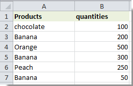
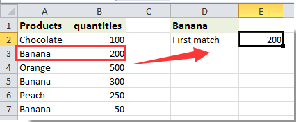
假設您有兩列產品和數量,如下圖所示。 為了快速找出第一根或第二根香蕉的數量,您會怎麼做?

這裡的vlookup函數可以幫助您解決此問題。 在本文中,我們將向您展示如何使用Excel中的Vlookup函數vlookup查找第一個,第二個或第n個匹配值。

Vlookup使用公式在Excel中查找第一個,第二個或第n個匹配值

使用Kutools for Excel輕鬆vlookup在Excel中查找第一個匹配值


Vlookup在Excel中查找第一個,第二個或第n個匹配值

請執行以下操作以在Excel中找到第一個,第二個或第n個匹配值。

1.在單元格D1中,輸入要查看的條件,在這裡輸入“香蕉”。

2.在這裡,我們將找到香蕉的第一個匹配值。 選擇一個空白單元格,例如E2,複製並粘貼公式 =INDEX($B$2:$B$6,MATCH(TRUE,EXACT($D$1,$A$2:$A$6),0)) 進入編輯欄,然後按 按Ctrl + 轉移 + Enter 鍵同時。

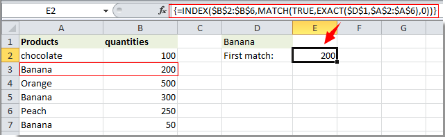
備註:在此公式中,$ B $ 2:$ B $ 6是匹配值的範圍; $ A $ 2:$ A $ 6是具有所有vlookup條件的範圍; $ D $ 1是包含指定vlookup條件的單元格。

然後,您將在單元格E2中獲得香蕉的第一個匹配值。 使用此公式,您只能根據您的條件獲得第一個對應的值。

要獲取第n個相對值,可以應用以下公式: =INDEX($B$2:$B$6,SMALL(IF($D$1=$A$2:$A$6,ROW($A$2:$A$6)-ROW($A$2)+1),1)) + 按Ctrl + 轉移 + Enter 鍵在一起,此公式將返回第一個匹配的值。

筆記:

1.要找到第二個匹配值,請將上面的公式更改為 =INDEX($B$2:$B$6,SMALL(IF($D$1=$A$2:$A$6,ROW($A$2:$A$6)-ROW($A$2)+1),2)),然後按 按Ctrl + 轉移 + Enter 同時鍵。 看截圖:

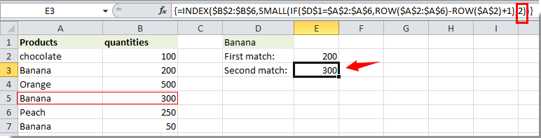
2.上式中的最後一個數字表示vlookup條件的第n個匹配值。 如果將其更改為3,它將獲得第三個匹配值,並更改為n,將找到第n個匹配值。


Vlookup使用Kutools for Excel在Excel中查找第一個匹配值

Y您無需記住公式即可輕鬆地在Excel中找到第一個匹配值 在列表中查找值 公式的 Excel的Kutools.

申請前 Excel的Kutools首先下載並安裝.

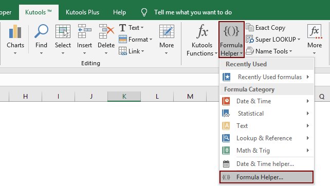
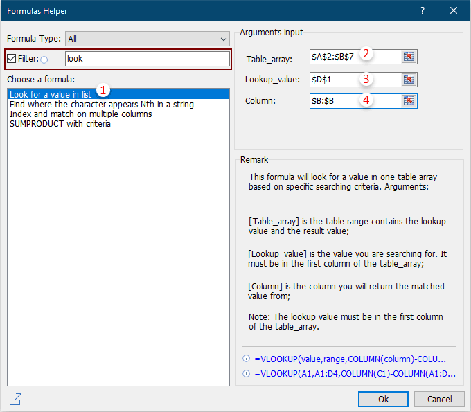
1.選擇一個單元格以查找第一個匹配值(例如單元格E2),然後單擊 庫工具 > 公式助手 > 公式助手。 看截圖:

3。 在裡面 公式助手 對話框,請進行如下配置:

  • 3.1在 選擇一個公式 框,找到並選擇 在列表中查找值;
    保養竅門:您可以檢查 篩選 框,在文本框中輸入特定單詞以快速過濾公式。
  • 3.2在 表格數組 框,選擇 包含第一個匹配值的表格。;
  • 3.2在 查找值 框,選擇包含 標準 您將基於返回第一個值;
  • 3.3在 框,指定您要從中返回匹配值的列。 或者,您可以根據需要直接在文本框中輸入列號。
  • 3.4點擊 OK 按鈕。 看截圖:

現在,將基於下拉列表選擇在單元格C10中自動填充相應的單元格值。

  如果您想免費試用(30天)此實用程序, 請點擊下載,然後按照上述步驟進行操作。

最佳辦公生產力工具

🤖 Kutools 人工智慧助手:基於以下內容徹底改變數據分析: 智慧執行   |  生成代碼  |  建立自訂公式  |  分析數據並產生圖表  |  呼叫 Kutools 函數...
熱門特色: 尋找、突出顯示或識別重複項   |  刪除空白行   |  合併列或儲存格而不遺失數據   |   沒有公式的回合 ...
超級查詢: 多條件VLookup    多值VLookup  |   跨多個工作表的 VLookup   |   模糊查詢 ....
高級下拉列表: 快速建立下拉列表   |  依賴下拉列表   |  多選下拉列表 ....
欄目經理: 新增特定數量的列  |  移動列  |  切換隱藏列的可見性狀態  |  比較範圍和列 ...
特色功能: 網格焦點   |  設計圖   |   大方程式酒吧    工作簿和工作表管理器   |  資源庫 (自動文字)   |  日期選擇器   |  合併工作表   |  加密/解密單元格    按清單發送電子郵件   |  超級濾鏡   |   特殊過濾器 (過濾粗體/斜體/刪除線...)...
前 15 個工具集12 文本 工具 (添加文本, 刪除字符,...)   |   50+ 圖表 類型 (甘特圖,...)   |   40+ 實用 公式 (根據生日計算年齡,...)   |   19 插入 工具 (插入二維碼, 從路徑插入圖片,...)   |   12 轉化 工具 (數字到單詞, 貨幣兌換,...)   |   7 合併與拆分 工具 (高級合併行, 分裂細胞,...)   |   ... 和更多

使用 Kutools for Excel 增強您的 Excel 技能,體驗前所未有的效率。 Kutools for Excel 提供了 300 多種進階功能來提高生產力並節省時間。  點擊此處獲取您最需要的功能...

產品描述


Office選項卡為Office帶來了選項卡式界面,使您的工作更加輕鬆

  • 在Word,Excel,PowerPoint中啟用選項卡式編輯和閱讀,發布者,Access,Visio和Project。
  • 在同一窗口的新選項卡中而不是在新窗口中打開並創建多個文檔。
  • 將您的工作效率提高 50%,每天為您減少數百次鼠標點擊!
Comments (43)
No ratings yet. Be the first to rate!
This comment was minimized by the moderator on the site
You only return first match with VLOOKUP so your article "How To Vlookup Find The First, 2nd Or Nth Match Value In Excel?" does not make any sense....
This comment was minimized by the moderator on the site
Hi Sima,
"VLOOKUP" is a Google search term, so I used it as a keyword for the article title. The main operation of this article is to lookup values. I'm sorry for the misunderstanding.
This comment was minimized by the moderator on the site
What if the next record on col b is a duplicate how do ignore duplicate? Let's Banana has quantities of 200 twice? Can you please help me figure out how to ignore the duplicate?
This comment was minimized by the moderator on the site
Cna anybody Explain the small function with the IF statement for me please? I don't really understand how that array works :(
This comment was minimized by the moderator on the site
The following formulas works perfect for me:
(a) or(b) =IF(H8='Raw Data'!B4,INDEX('Raw Data'!H6:H20,SMALL(IF(C18='Raw Data'!B6:B20,ROW('Raw Data'!B6:B20)-ROW('Raw Data'!B6:B20)+1),1)))

However, I have encountered a problem where there are 7 sets of the same criteria but in different columns:(1) can the above formula (a) be repeated and search in a different cells in a single formula and(2) the above formula (b) only allows up to two sets of the similar search with matched value result but when trying for the third set in the formula as showed below, Microsoft Excel appeared as "You've entered too many arguments for this function."
=<span style="letter-spacing: 0.2px; color: inherit; font-family: inherit; font-style: inherit; font-variant-ligatures: inherit; font-variant-caps: inherit; font-weight: inherit;">IF(H8='Raw Data'!J4,INDEX('Raw Data'!P6:P20,SMALL(IF(C18='Raw Data'!J6:J20,ROW('Raw Data'!J6:J20)-ROW('Raw Data'!J6:J20)+1),1))),</span>
This comment was minimized by the moderator on the site
What do Ctrl + Shift + Enter do?? At the beginning I didn'
This comment was minimized by the moderator on the site
Hi,An array formula needs to hit the Ctrl + Shift + Enter keys simultaneously to get the correct result.
This comment was minimized by the moderator on the site
I have a scenario... How do I get last price of anything for reference... Example: Banana first price was 200... While purchasing for second time; I need to display 200 in my expected price cell and then if I buy that on the day at 220, I will put this value manually as 220... Whenever next time I will buy banana; I need to display 220 from the last purchase price
This comment was minimized by the moderator on the site
Try =INDEX($B$2:$B$6,XMATCH(TRUE,EXACT($D$1,$A$2:$A$6),0,-1))

This is essentially reversing the search order and returning the first match using the XMATCH function.

Better late than never, hopefully helps someone :)
This comment was minimized by the moderator on the site
Perfect explanation, thanks.
This comment was minimized by the moderator on the site
If the first or any of the other entry's for 'banana' column B was blank cell, of which I don't require this number, what changes are required to this formula to skip blank cell in column B.
This comment was minimized by the moderator on the site
Sorry I am using this formula
=INDEX($B$2:$B$6,SMALL(IF($D$1=$A$2:$A$6,ROW($A$2:$A$6)-ROW($A$2)+1),1))
This comment was minimized by the moderator on the site
SOLVED:
=SMALL(IF(A2:A7=D1,IF(B2:B7<>"",B2:B7)),1)

If 2nd or 3rd number required exchange ),1) to 2 or 3

This formula does not require index, as it directly looks at the value in Cell
This comment was minimized by the moderator on the site
Correction to previous formula:
The value was reading either the lesser or greater.

Updated formula
=INDEX($B$2:$B$7,SMALL(IF($A2:$A6=$D$1,IF($B$2:$B$7<>"",ROW($A2:$A6)-ROW($A2)+1)),1))

This skips blank cell and places value of non blank cell. Replace +1 with +2 or +3 for 2nd or 3rd value
This comment was minimized by the moderator on the site
And if you want the last, second last, nth last just add a counter (count the number of events already hapenned) to the end and subtract it by 0,1,n respectively.

Thank you so much! I was searching for this for a long time
This comment was minimized by the moderator on the site
Good Day,
Sorry can't help you with this yet. Thank you for your comment.
This comment was minimized by the moderator on the site
Is it possible to find an average of the non-unique data. Or would it be possible to have a list dropdown on the cell of the various values?
This comment was minimized by the moderator on the site
Good Day,
Sorry can't help you with this yet. Thank you for your comment.
There are no comments posted here yet
Load More
Please leave your comments in English
Posting as Guest
×
Rate this post:
0   Characters
Suggested Locations