如何在 Excel 中使用條件格式突顯超過 30 天的舊日期？

作者孫修改日期2025-08-07

當您在 Excel 中處理日期清單時，經常需要突顯比今天早超過 30 天的日期。手動識別這些日期不僅耗時，還容易出錯，尤其在面對大型資料集時更是如此。本指南為您介紹多種高效方法，協助您輕鬆突顯或管理超過 30 天的日期：包括運用條件格式自動標示、透過輔助公式進行排序與標記、針對大型或動態範圍使用 VBA 巨集，甚至善用專業工具簡化整體工作流程。掌握這些技巧，您將能快速辨識逾期日期、有效追蹤截止期限，並從容管理具時效性的資料。

使用使用條件格式突顯超過 30 天的日期
 利用強大工具輕鬆選取並突顯早於特定日期的日期
 透過 VBA 巨集自動突顯超過 30 天的日期
 使用輔助欄位公式標記超過 30 天的日期

使用使用條件格式突顯超過 30 天的日期

Excel 的「條件式格式」功能可自動突顯所選區域中早於 30 天的日期，非常適合用於追蹤逾期任務、管理截止期限，或根據項目年齡進行優先排序。請依照以下詳細步驟操作：

1. 選取包含日期的範圍，然後前往開始 > 使用條件格式 > 新增規則。請參閱螢幕截圖：

點擊「開始」>「條件式格式設定」>「新增規則」的螢幕截圖

2. 在「新增格式設定規則」對話方塊中，進行下列設定：

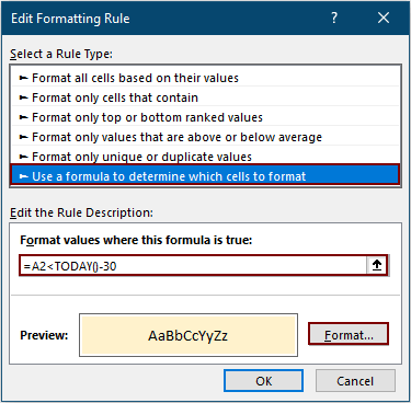
2.1) 選擇使用公式來決定要格式化的儲存格（位於「規則類型」選項下方）。
2.2) 在標示為「當此公式為真時格式化數值」的方框中輸入此公式：
=A2<TODAY()-30
2.3) 按一下格式，指定用於突顯舊日期的填充顏色。
2.4) 按一下確定以確認並套用規則。請參閱螢幕截圖：

注意：此公式中的 A2 應為您所選區域的左上角儲存格，而 30 則代表天數門檻值。兩者皆可依需求調整：若您的資料並非從 A2 開始，請相應更新儲存格參照，並確保其指向範圍的第一列。

設定完成後，Excel 會以您指定的顏色突顯範圍內所有早於今天超過 30 天的日期，立即引起您對可能需立即處理項目的注意。

所有早於今天30天以上的日期都會被醒目提示

提示：此公式會將每個儲存格的日期與 TODAY()減去 30 後的結果進行比較。若您想突顯其他時間範圍（例如 60 天），只需將「30」替換為您偏好的數字即可！

若您的日期清單包含空白儲存格，可能會發現這些儲存格偶爾也被突顯。為避免突顯空白儲存格：

3. 重新選取您的日期範圍，然後依序前往開始 > 使用條件格式 > 管理規則。

點擊「開始」>「條件式格式設定」>「管理規則」的螢幕截圖

4. 在使用條件格式規則管理中，點擊新增規則，即可新增處理空白儲存格的規則。

點擊「新增規則」按鈕的螢幕截圖

5. 在「編輯格式設定規則」對話方塊中：

5.1) 選擇使用公式來決定要格式化的儲存格。
5.2) 輸入下列公式（若您的範圍不是從 A2 開始，請予以替換）：
=ISBLANK(A2)=TRUE
5.3) 按一下確定以確認。

6. 在規則管理中，務必為新規則勾選「符合時停止」核取方塊，確保空白儲存格不會受其他格式設定規則影響。立即點選確定完成設定！

勾選「符合條件時停止」核取方塊

結果：僅實際日期值且早於 30 天的儲存格會被突顯，空白儲存格將如預期般予以忽略。

僅醒目提示早於30天以上的日期，並排除空白儲存格

情境與提示：條件格式非常適合用於需要快速視覺化逾期項目的互動式儀表板或報表！但請注意，若套用範圍過大或格式規則過於複雜，可能會影響活頁簿效能。務必再次確認日期格式：此規則僅在儲存格被 Excel 識別為日期時才會生效。

利用強大工具輕鬆突顯早於特定日期的日期

若您需要一種快速且使用者友善的方式，來選取並突顯早於特定日期的資料（例如用於自訂報表或手動批次作業），選擇指定單元格（位於）Kutools for Excel 中）提供了高效解決方案！只需點擊幾下，即可立即選取所有早於指定日期的儲存格，並依需求輕鬆完成突顯或後續處理。

Kutools for Excel 提供超過 300 項進階功能，簡化複雜作業，提升創造力與效率。整合 AI 功能，Kutools 能精準自動化各項任務，讓資料管理輕鬆無負擔。Kutools for Excel 的詳細資訊…… 免費試用……

1. 選取日期儲存格，按一下 Kutools > 選取 > 選擇指定單元格。

點擊 Kutools 的「選取特定儲存格」功能

2. 在選擇指定單元格對話方塊中，您需要：

2.1) 選取儲存格（位於）選擇類型區段中）。
2.2) 從小於（位於）指定類型下拉選單）中選擇，並在方框中輸入截止日期（例如 30 天前或特定日期）。
2.3) 按一下確定，即可選取所有符合條件的日期儲存格。
2.4) 在確認選取數量後，按一下資訊對話方塊中的確定以繼續。

在「選取特定儲存格」對話框中設定選項

3. 選取相關日期後，可前往開始> 填充顏色，套用色彩以視覺化突顯所需項目。

想免費試用此工具 30 天嗎？立即下載，並依照上述步驟操作！

透過 VBA 巨集自動突顯超過 30 天的日期

若您正在處理大型資料集，或經常需要突顯相對於今天的日期，VBA 巨集能有效自動化此流程。當您面對範圍極大、需反覆更新突顯效果，或需先清除先前格式再套用新突顯時，此方法尤其實用。

1. 開啟您要套用醒目提示的 Excel 工作表，然後按一下開發人員工具＞Visual Basic，即可進入 VBA 編輯器。若未顯示「開發人員」索引標籤，請先至 Excel 選項中啟用。接著在 VBA 視窗中，點選插入＞模組。

Sub HighlightOldDates()
    Dim WorkRng As Range
    Dim Rng As Range
    Dim xTitleId As String
    
    xTitleId = "KutoolsforExcel"
    On Error Resume Next
    Set WorkRng = Application.Selection
    Set WorkRng = Application.InputBox("Select the range to check for old dates:", xTitleId, WorkRng.Address, Type:=8)
    
    Application.ScreenUpdating = False
    ' Optional: Clear previous background coloring
    WorkRng.Interior.ColorIndex = xlNone
    
    For Each Rng In WorkRng
        If IsDate(Rng.Value) Then
            If Rng.Value < Date - 30 Then
                Rng.Interior.Color = vbYellow ' Or choose any other color you prefer
            End If
        End If
    Next
    
    Application.ScreenUpdating = True
    MsgBox "Highlighting complete.", vbInformation, xTitleId
End Sub

2. 執行巨集時，請點選執行（VBA 編輯器中的綠色三角形按鈕），或在選取模組後按下 F5. 系統將立即彈出對話方塊，提示您選取要分析的日期範圍。巨集會自動清除先前的填充顏色，並將超過 30 天的日期儲存格以黃色醒目標示（您可依需求自行調整顏色）！

實務注意事項：－此 VBA 解決方案非常適合處理重複性任務或分析大型試算表。－執行 VBA 程式碼前，務必先儲存活頁簿，尤其是使用會變更格式的巨集時。－VBA 巨集需搭配啟用巨集的活頁簿（.xlsm）及啟用巨集的設定；若為共用或線上活頁簿，建議改用上述其他方法。

疑難排解：如果巨集似乎無法運作，請先確認日期儲存格格式正確，並仔細檢查所選區域。若其中包含非日期值，系統將自動忽略。

使用輔助欄位與公式標記超過 30 天的日期

若需更靈活地識別舊日期（例如用於篩選、排序或觸發其他動作），可搭配使用輔助欄位與 Excel 公式。當您需要進一步處理或分析已標記的結果（而不僅僅是變更儲存格顏色）時，此方法尤其實用。

1. 在您的日期清單旁插入一個新欄位（例如，若日期從 A 欄開始，請新增 B 欄並標示為「逾期標記」）。接著，在輔助欄位的第一列（例如 B2）輸入下列公式：

=A2<TODAY()-30

此公式會檢查 A2 儲存格中的日期是否早於今天超過 30 天。若條件成立，則傳回 TRUE；否則，傳回 FALSE。

2. 按下 Enter 套用公式後，將其快速複製至整個數據區域！選取 B2 儲存格，向下拖曳填滿控點，或在鄰近有資料時直接按兩下控點，即可輕鬆完成。

3. 完成後，您即可根據 TRUE/FALSE 值進行篩選或排序，其中 TRUE 的列即為日期超過 30 天的項目。

實際應用：您現在即可篩選資料、套用其他格式規則，或將此標記欄位運用於進一步的計算與自動化流程中。當您在日期逾期時需執行額外步驟（例如產生報表或傳送通知），此方法格外高效！

提示：只需調整公式中的 30，即可設定不同的閾值。務必確保公式與您的實際數據區域相符！

最佳適用情境：此方法提供細緻的控制與可稽核性，非常適合用於處理大型資料集，或整合至自動化工作流程中。

選擇合適的醒目提示方法時，請考量您的需求：使用條件格式最適合動態視覺提示；輔助欄位可支援進階處理；篩選/排序最適合快速檢閱且不需變更工作表；VBA 非常適合重複性或高頻率任務；而 Kutools for Excel 則能提供快速且彈性的選取功能，適用於手動或批次作業。務必留意日期格式與活頁簿共用限制，並在套用變更前儲存檔案，特別是使用 VBA 或增益集工具時。結合多種方法可為複雜工作流程帶來強大的解決方案。

在 Excel 中標示小於／大於今天的條件格式日期
本教學將詳細說明如何運用 TODAY 函數搭配條件格式，輕鬆突顯 Excel 中的截止日期或未來日期！

在 Excel 條件格式中忽略空白或零值儲存格
假設您有一份包含零值或空白儲存格的資料清單，想套用條件格式卻又希望忽略這些空白或零值儲存格，該如何處理？本文將為您提供實用解法！

將條件格式規則複製到其他工作表／活頁簿
例如，您已根據第二欄（水果欄）中的重複儲存格對整列進行條件式突顯，並對第四欄（金額欄）中的前三名數值套用色彩標示（如下方螢幕截圖所示）。現在，您希望將此範圍的條件格式規則複製到其他工作表／活頁簿。本文提供兩種實用方法供您參考！

在 Excel 中根據文字長度突顯儲存格
假設您正在處理一份包含文字字串清單的工作表，並希望突顯所有文字長度超過 15 的儲存格。本文將為您介紹幾種在 Excel 中輕鬆達成此任務的實用方法！

最佳 Office 生產力工具

🤖	KUTOOLS AI 助手：基於以下內容徹底革新數據分析：智慧執行｜產生程式碼｜建立自訂公式｜分析資料並產生圖表｜呼叫增強函數……
	熱門功能：尋找、醒目提示或標記重複值｜刪除空白行｜合併列或儲存格而不遺失資料｜不使用公式的四捨五入……
	高級 LOOKUP：多重條件 VLookup ｜多重數值 VLookup ｜跨多個工作表 VLookup ｜模糊查找……
	高級下拉列表：快速建立下拉式清單｜相依式下拉式清單｜多選下拉式清單……
	欄位管理員：新增指定數量的欄位｜移動欄位｜切換隱藏欄位的可見狀態｜比較範圍與欄位……
	精選功能：網格聚焦｜設計視圖｜增強編輯欄｜工作簿與工作表管理員｜資源庫（自動文字）｜日期提取｜合併工作表｜加密／解密儲存格｜依清單傳送電子郵件｜超級篩選｜特殊篩選（篩選粗體儲存格／斜體／刪除線……） ......
	頂尖 15 工具組：12 文字工具（添加文本，刪除特定字符，……）｜ 50+ 圖表類型（甘特圖，……）｜ 40+ 實用公式（基於生日計算年齡，……）｜ 19 插入工具（插入二維碼，從路徑插入圖片，……）｜ 12 轉換工具（金額轉大寫，匯率轉換，……）｜ 7 合併和拆分工具（高級合併行，分割儲存格，……）｜……以及更多